Geometric effects in the design of catalytic converters in car exhaust pipes

Abstract

Introduction

We solve the gas dynamics (Euler) equations, augmented by adding a fourth equation governing the fraction of unburnt gas, in a number of cylindrically symmetric configurations of the pipe system.

Case description

The purpose is to test several duct profiles to see which one favors a higher reduction of the residual noxious gases, at the end of a car’s exhaust pipe.

Discussion and evaluation

It is found that this purely geometric factor does play a role in the environment’s purification accomplished by the catalytic converter. This is possibly due to the longer time spent by the noxious gases resident inside the device when this has certain profiles, though at the price of a little higher temperature attained.

Conclusions

It seems that geometric factors play a role in reducing cars’ noxious gases by means of catalytic converters. A more precise analysis should be formulated as a mathematical inverse problem.

Background

An important issue related to the problem of air pollution is the functioning of an increasing number of cars, fed by traditional fuels. In the 2003 review paper [11], it was pointed out that in the previous 60 years the number of vehicles has increased from about 40 to over 700 millions, predicting a further increase of several hundreds of millions in the forthcoming years.

A possible remediation, capable to control and hence to limit harmful effects of air pollution has been for many years represented by the adoption of suitable “catalytic converters”. Indeed, a few periodicals and many books exist which address specifically these issues.

A catalytic converter is a device capable to control the car exhaust emissions, transforming the toxic gases generated by internal combustion engines into less toxic or even harmless inert products by means of catalytic oxidation and/or reduction.

Catalytic phenomena are also important in many other fields, such as industrial chemistry, combustion science, chemical engineering, besides automotive engineering and environmental sciences, as is witnessed by a number of specialized periodicals fully devoted to the them.

“Two-way” converters combine oxygen with carbon monoxide (CO) and various unburnt hydrocarbons to produce carbon dioxide (CO₂) and water vapor, respectively, through oxidation reactions. For instance, 2 CO+O₂→2 CO₂. “Three-way” devices, transform, in addition, oxides of nitrogen (nitric oxide, NO, and nitrogen dioxide, NO₂) reducing them to nitrogen, N₂. The catalytic devices contain a catalyst support whose core is a ceramic monolith with a honeycomb structure, the catalyst consisting of some precious metal such as platinum (good for both, oxidation and reduction), or palladium (good for oxidation), or rhodium (good for reduction).

A review written in 2014 [7] reports advances made on automotive catalysts over the previous four decades. Research work on this subject addresses several aspects, such as numerical models, computational fluid dynamic models, design of catalytic converters, laboratory experiments, and development of catalytic materials; see also [15] for a review concerning works on automobile catalytic converters carried out up to about 2013, as well as future perspectives. Some relevant results concerning autothermal catalytic combustion can be found in the recent works [4–6].

This paper concerns the design of catalytic converters. More specifically, its purpose is to attempt to devise the optimal shape of a car’s exhaust system where a catalytic converter is lodged, aiming at obtaining the smallest residual noxious gas concentration at the end of the pipe. We consider a simple one-dimensional model where only a single gas species, undergoing a phase change, since the burnt and unburnt phases coexist.

The chemical reactions occurring inside the catalytic device are also ignored. Despite its simplicity, this model, apparently, provides significant results, in good agreement with the experimental measurements accomplished by the company Magneti Marelli S.p.A.

We solved a system of four inhomogeneous coupled gas dynamics equations, namely the (three) Euler equations with some source terms, plus a fourth equation which describes the dynamical behavior of the unburnt residual (noxious) gas’ fraction, in a duct of variable cross-section. The source terms are due to a number of physical and chemical effects, such as gas-wall friction, thermal exchanges, and chemical reactions. From the mathematical standpoint, this is a system of four nonlinear hyperbolic partial differential equations termed balance laws, rather than conservation laws, since the sources destroy the basic conservation properties of the classical compressible Euler equations of gas dynamics. The system of equations is appropriately “closed” using an appropriate state equation, and is supplemented with initial and boundary conditions.

Needless to say, the fully nonlinear character of such balance laws makes their theory as well as their numerical treatment highly nontrivial. In particular, adding source terms to conservation laws implies that successful algorithms like finite volumes and Godunov schemes do not work well as they do with conservation laws, since they are conservative schemes. A better numerical treatment has been realized resorting to certain kinetic schemes [1, 13], and in particular to the so-called AHOp (Asymptotic High-Order) finite difference schemes, developed in [2, 3].

The aforementioned system of equations can be simplified taking into account the cylindrical geometry of the device, even though it has a variable cross-section. This setting includes pipes and few components such as precatalyzer, catalyzer, and mufflers. In fact, the aforementioned equations can be averaged over each section of the system, thus reducing the space dimensionality of the mathematical problem from three to one space dimensions [13]. We used real data, provided by the Magneti Marelli at the time when the Masters thesis in [13] was written.

We should point out two sensible issues, which represent limitations of the model. One is that, in general, there are many reacting species in the flow of the exhaust gas through a given catalytic converter, while here we consider a simplified model where only a single gas species is present. The other is that the reactions actually take place on the surface of the catalyst, while the temperature we used in the reaction rate is the gas temperature (and not the temperature of the surface of the catalyst). These can be considered as some kind of approximations but, nevertheless, our results match well with the experimental data provided by Magneti Marelli [13].

In this paper, we have implemented some well-established algorithms, namely an AHO2 scheme, to solve the four aforementioned balance laws in a number of configurations of the pipe’s profile. Thus, we explored the effects of the pipe geometry on the residual fraction of noxious gas at the end of the pipe, that is the amount of the pollutant which is injected into the environment (into the atmosphere).

The main results are the following. First of all, the original configuration adopted by Magneti Marelli turned out to be rather satisfactory, close to the best that one could design. Playing with the geometry, however, it is possible to identify some profiles for which a further reduction, up to about 6%, of the residual gas can be obtained. We speculate that this positive effect of the geometry might be due to the fact that some ripples, some corrugation, in the duct’s profile imply a longer time for the gas to linger around the catalytic material, thus increasing the efficiency of the latter. The price to pay for this is that the maximum temperature attained by the gas turns out to be a little higher than in the case of the Magneti Marelli’s device.

Here is the plan of the paper. In section “Case description: The basic problem and its mathematical formulation”, the basic problem is described, and a mathematical model is formulated. We omit the detailed description of the numerical methods we used, i.e., of the numerical treatment of balance laws, since this is not the focus of the present investigations, besides being not new. The interested reader might also consult, e.g., [8, 10, 16]. In section “Discussion and evaluation: Numerical results obtained varying the duct’s geometry”, the numerical results, obtained varying the pipe’s geometry in a number of ways, are shown, and some conclusions are then drawn in the final section “Conclusions”.

Case description: The basic problem and its mathematical formulation

Here is the basic mathematical problem and its mathematical formulation. A catalytic converter is a device whose purpose is to filter out, possibly to eliminate, the noxious gases flowing into the environment from the end of the cars’ exhaust pipes, Fig. 1

Fig. 1

Various parts of a catalyzer system. (By courtesy of Encyclopaedia Britannica, Inc., copyright 2006; used with permission)

A mathematical model can be constructed for a single gas species, which undergoes a phase change (since burnt and unburnt fractions will coexist), along the following lines:

• the Euler equations of gas dynamics have to be supplemented with an additional equation, which describes the time evolution of the fraction of noxious gas;

• a simplified (one-dimensional) geometry can be adopted;

• a closure equation is needed;

• suitable initial and boundary conditions are prescribed.

The three classical Euler equations of gas dynamics, averaged over the cross section, A=A(x), are

$$ \left\{ \begin{array}{ll} \partial_{t}(A \rho) + \partial_{x}(A \rho u) = 0 & \ \ \text{(mass conservation)} \\ \partial_{t}(A \rho u) + \partial_{x}(A(\rho u^{2} + p)) = 0 & \ \ \text{(momentum conservation)} \\ \partial_{t}(A E) + \partial_{x}(A u (E + p)) = 0 & \ \ \text{(energy conservation)}. \\ \end{array} \right. $$

(1)

Here ρ,u,p, and E are density, velocity, pressure, and total energy, E:=ρe+ρu²/2, being e the specific internal energy (the internal energy per unit mass), and ρu²/2 the kinetic energy. Since we have three equations but four unknowns, a closure relation is needed: If we assume the gas to be ideal and the flow homentropic within the pipe, then p=(γ−1)ρe, with γ=c_p/c_v the specific heat ratio (the adiabatic exponent), c_p and c_v the specific heats (1<γ<2). Hence, we can write $E = \frac {p}{\gamma - 1} + \frac {1}{2} \rho u^{2}$.

Moreover, in case of an exhaust pipe, we should take into account some additional phenomena, as follows.

• Friction with the pipe’s wall: When a fluid travels through a pipe, a friction develops as a hydraulic resistance due to transfer of momentum to the solid wall. Thus, a force is exerted on each surface unit of the solid wall. Mathematically, this amounts to introduce a term like

  $$ - C_{f} \, w \, \rho \, \frac{u^{2}}{2}, $$

  (2)

  that can be obtained from the so-called Darcy’s empirical formula [12], on the right-hand side of the moment equation. The numerical value of the friction coefficient, C_f, that in the literature is given by the Darcy-Weisbach equation, was obtained by a series of tests conducted by Magneti Marelli [13]; w in general a function of x, is the perimeter of the duct section.

• Friction with the honeycomb structure of the catalyzer: A honeycomb structure for the catalyzing (ceramic) material is chosen to maximize the surface exposed to the noxious gas of the chemical reagents, Fig. 2. It implies, however, an additional obstacle to the gas flow through the pipe, hence giving rise to a decrease of speed and pressure (due to a resistance exerted on the gas). From the mathematical standpoint, this amounts to introduce a term like

  $$ - C \rho u $$

  (3)

  Fig. 2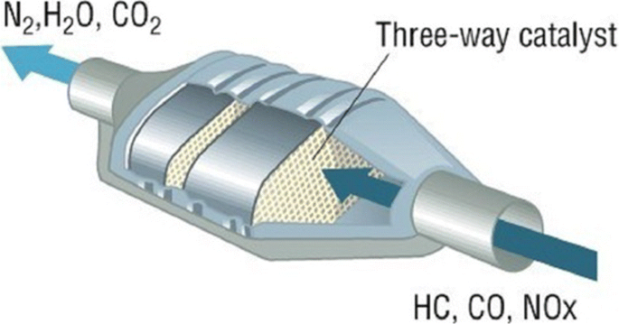

  

  A three-way catalytic converter. Note the honeycomb structure. (By courtesy of AA1Car; reprinted with permission)

  again on the right-hand side of the moment equation. This choice is empirical, and the friction coefficient, C, was determined experimentally [13]. Usually, some form of the Darcy’s law is assumed for gas flowing through porous media, at least when the regime is laminar.

• Heat exchanged by conduction: Thermal exchanges between gas and external environment are governed by Newton’s law, according to which the heat transfer between a surface (the wall) at temperature θ_w and the fluid at temperature θ, is given by the quantity

  $$ - w h (\theta - \theta_w), $$

  (4)

  where w=w(x) is the duct’s perimeter (Note that $w = 2 \sqrt {\pi A}$, in terms of the cross sectional area, A), h (evaluated experimentally [13]) is the heat transfer coefficient. This term will be introduced on the right-hand side of the equation for the energy conservation.

  These terms affect the right-hand sides of Euler equations. Our model must include, in addition, a fourth equation, which represents “the continuity equation for the unburnt gas”. Consider two states, the burnt and the unburnt gas. The unburnt gas is transformed into burnt gas through

• A chemical reaction, governed by the Arrhenius’ empirical law,

  $$ K(\theta) = K_{0} \exp(- E^+/R \theta). $$

  (5)

  widely used in chemical kinetics, where K₀ represents a (constant) reaction rate and E⁺ is the activation energy, and R is the gas constant [14]. Therefore, we augment the previous system adding to it the equation

  $$ \partial_{t}(A q_{0} \rho z) + \partial_{x}(A u q_{0} \rho z) = - q_{0} \rho z K(\theta), $$

  (6)

  where q₀ represents the amount of released heat per mass unity, and z=z(x,t) denotes the fraction of unburnt gas. Clearly, 0≤z(x,t)≤1, and 1−z(x,t) represents the burnt gas fraction.

  Adding such an equation, however, the first three equations have to be further modified, since the total energy becomes

  $$ E = \rho e + \rho \frac{u^{2}}{2} + q_{0} \rho z. $$

  (7)

  This relation represents a balance among internal energy, kinetic energy, and energy involved in the burnt gas fraction. Note that the chemical reaction appears here, in such last equation. Finally, the system of four equations (balance laws) will be

  $$ \left\{ \begin{array}{ll} \partial_{t}(A \rho) + \partial_{x}(A \rho u) = 0 \\ \partial_{t}(A \rho u) + \partial_{x}(A (\rho u^{2} + p)) = - C_{f} w \rho u^2/2 - C \rho u \\ \partial_{t}(A E) + \partial_{x}(A u (E + p)) = - w h (\theta - \theta_w) \\ \partial_{t}(A q_{0} \rho z) + \partial_{x}(A u q_{0} \rho z) = - q_{0} \rho z K(\theta), \end{array} \right. $$

  (8)

  Extracting the cross-section term, A, and setting q:=ρu and Z:=q₀ρz, we can write this system as

  $$ \left\{ \begin{array}{ll} \partial_{t} \rho + \partial_{x} q = - \frac{A'}{A} q \\ \partial_{t} q + \partial_{x} \left(\frac{q^{2}}{\rho} + p \right) = - \frac{A'}{A} \left(\frac{q^{2}}{\rho} + p \right) - \frac{C_{f} w}{2 A} \frac{q^{2}}{\rho} - \frac{C}{A} q \\ \partial_{t} E + \partial_{x}(u (E + p)) = - \frac{A'}{A} u (E + p) - \frac{w h}{A} (\theta - \theta_w) \\ \partial_{t} Z + \partial_{x}\left(\frac{q}{\rho} Z\right) = - \frac{A'}{A} \frac{q}{\rho} Z - \frac{1}{A} Z K(\theta), \end{array} \right. $$

  (9)

  and finally, setting for short a:=A^′(x)/A(x),

  $$ \left\{ \begin{array}{ll} \partial_{t} \rho + \partial_{x} q = - a q \\ \partial_{t} q + \partial_{x} \left[\frac{q^{2}}{2 \rho} (3 - \gamma) + (\gamma - 1) (E - Z) \right] \\ \phantom{aaaaa} = - a \left[\frac{q^{2}}{2 \rho} (3 - \gamma) + (\gamma - 1) (E - Z) \right] - \frac{C_{f} w}{2 A} \frac{q^{2}}{\rho} - \frac{C}{A} q \\ \partial_{t} E + \partial_{x} \left[\frac{q}{\rho} \left(\gamma E - (\gamma - 1) \frac{q^{2}}{2 \rho} - (\gamma - 1) Z \right) \right] \\ \phantom{aaaaa} = - a \left[\frac{q}{\rho} \left(\gamma E - (\gamma - 1) \frac{q^{2}}{2 \rho} - (\gamma - 1) Z \right) \right] - \frac{w h}{A} (\theta - \theta_w) \\ \partial_{t} Z + \partial_{x}\left(\frac{q}{\rho} Z\right) = - a \frac{q}{\rho} Z - \frac{1}{A} Z K(\theta). \end{array} \right. $$

  (10)

  The temperature θ can be evaluated in terms of ρ,q,E and Z as

  $$ \theta = c_{v}^{-1} \left(\frac{E}{\rho} - \frac{q^{2}}{2 \rho^{2}} - \frac{Z}{\rho} \right), $$

  (11)

  or simply as $\theta = c_{v}^{-1} e$. In fact, compare

  $$ p = \rho R \theta = (c_{p} - c_v) \rho \theta = (\gamma - 1) c_{v} \rho \theta, $$

  (12)

  valid for an ideal gas, with

  $$ p = (\gamma - 1) \rho e. $$

  (13)

  Note that a variable cross-section acts on the system as a source term. Indeed, this is what happens always when inhomogeneities affect the flux in conservation laws [9]. The source depends also on x, due to the area terms and the perimeter, w. Setting

  $$ U := \left(\rho,\rho u,E,q_{0} \rho z \right)^{T} \equiv (\rho,q,E,Z)^{T}, $$

  (14)

  this system can be conveniently rewritten in vector form as

  $$ \partial_{t} U + \partial_{x}(F(U)) = S(U,x). $$

  (15)

  Since the duct is located in 0≤x≤L, the problem to solve is

  $$ \left\{ \begin{array}{ll} \partial_tU + \partial_{x}(F(U)) = S(U,x), \quad (x,t) \in (0,L) \times (0,T] \\ U(x,0) = U_{0}(x), \quad x \in (0,L), \end{array} \right. $$

  (16)

  being U, U₀(x), F(U), and S(U,x) four-dimensional vectors. Suitable initial and boundary conditions have to be prescribed. Throughout the paper, we used the following ones:

  $$ \left\{ \begin{array}{lll} \rho(x,0) = 1.21 \, Kg/m^{3}; & \rho(0,t) = 1 \, Kg/m^{3}; \\ u(x,0) = 413.22 \, m/s; & u(0,t) = 600 \, m/s; \\ \theta(x,0) = 295 \, ^oC; & \theta(0,t) = 800 \, ^oC; \\ p(x,0) = 1.0247 \times 10^{5} \, Pa; & p(0,t) = 2.2966 \times 10^{5} \, Pa; \\ z(x,0) = 0; & z(0,t) = 1. \end{array} \right. $$

  (17)

  Here, the variables x,t range over x∈[0,L] and t∈[0,T]. Prescribing ρ, u, θ, p, and z, for t=0 and at x=0, as here above, yields the values at t=0 and x=0 of all components of the vector U=U(x,t) defined in (14), recalling that e=p/((γ−1)ρ), while E can be obtained from either (7) or (11).

  There is no need to impose any boundary condition at x=L, since the flow is outward, that is it can be shown that the characteristics point out of the domain. Note that, from the last equations (concerning z), we assume that at the duct’s entrance the amount of unburnt gas be maximum, i.e., that the motor is unable to affect the gas’ emissions.

  The pipe system proposed by Magneti Marelli had all devices connected by joints whose profiles varied linearly with x, possibly discontinuously. The total fraction of unburnt gas at the end edge, x=L, of the exhaust pipe, at time T=1 s, was z(L,1)=0.7006, i.e., about 70%. Below, we show some results obtained by changing the forms of the connections between different sections of the system, as well as changing the whole geometric profile of the system. Since the profiles vary very smoothly and over short lengths, the flow remains subsonic and no effects due to converging or diverging nozzles is expected.

Discussion and evaluation: Numerical results obtained varying the duct’s geometry

Here are the numerical results obtained varying the duct’s geometry. The purpose of this section is to explore through numerical simulations a variety of the duct’s geometrical shapes, under which the noxious gases’ emissions at the end of the pipe could be reduced as much as possible. In fact, while the main chemical action which transforms the noxious gases into harmless products is due to the catalytic converters, the gas dynamics is also affected by the geometry (shape and volume) of the duct through which the gas flows. In particular, we first varied the duct’s profile without changing the device volume. All this only concerns the catalyzer’s geometry, since the mufflers do not affect the reduction of noxious gas.

A typical device, as that built by Magneti Marelli, consists of a precatalyzer, a catalyzer, and two mufflers; see Fig. 3 for illustration.

Fig. 3

Schematic duct’s geometry, like that of Magneti Marelli

Hereafter, we consider several possible connections, joining the various parts of the exhaust pipe, trying to optimize the catalyzer’s performance, also taking into account economical savings in terms of amount of material needed.

Starting from the typical Magneti Marelli’s device, where the various pieces are schematically connected as in Fig. 3, we first modify the joints, choosing for them linear, parabolic or cubic arcs, double parabolic arcs, and sinusoidal profiles. Finally, we will change completely the original shape of the catalyzer.

In Fig. 4 below, the main connecting points of a given configuration are shown. The radii of the pipe, the precatalyzer, and the catalyzer, are r₀=0.021 m, r₁=0.04 m, r₂=0.06 m, respectively.

Fig. 4

Catalyzers’ connecting points

To evaluate volumes, we used the formula for surfaces of revolution,

$$ V = \pi\int_{a}^{b} \left[f(x) \right]^{2} dx. $$

When these integrals were more elaborated, we evaluated them by means of symbolic manipulation, using Mathematica.

Below, we first describe several geometric configurations, and then summarize in a table the most relevant quantity, that is the total fraction of unburnt gas at the end of the pipe, at some reasonable time, z(L,T), obtained correspondingly.

(a) Straight lines connections. If a₁, a₂ are the two points delimiting the precatalyzer’s location, r₀ the duct’s radius, and r₁ that of the precatalyzer, considering joining them with straight lines, the variable radius will be given by

$$ r(x) = \frac{r_{1} - r_{0}}{a_{2} - a_{1}}(x - a_{1}) + r_{0}. $$

The catalyzer has radius r₂>r₁, see Figs. 4, 5.

Fig. 5

Duct’s section with linear connections between any two components

(b) Two parabolic arcs. The various components of the duct are connected by two parabolic arcs. The part between a₁ and a₂ with radius r₀ and r₁, respectively (Fig. 6) is connected by two generic parabolae, f(x)=ax²+bx+c and g(x)=αx²+βx+γ, such that f(a₁)=r₀, $f(\frac {a_{1} + a_{2}}{2}) = \frac {r_{0} + r_{1}}{2}$, f^′(a₁)=0, g(a₂)=r₁, $g(\frac {a_{1} + a_{2}}{2}) = \frac {r_{0} + r_{1}}{2}$, g^′(a₂)=0. From these, the six coefficients above can be obtained, hence the radii:

$$ f(x) = \frac{2 (r_{1} - r_{0})}{(a_{1} - a_{2})^{2}}x^{2} - 4 a_{1} \frac{(r_{1} - r_{0})}{(a_{1} -a_{2})^{2}} x + r_{0} + 2 a_{1}^{2} \frac{(r_{1} - r_{0})}{(a_{1} - a_{2})^{2}}, $$

$$ g(x) = \frac{2 (r_{0} - r_{1})}{(a_{1} - a_{2})^{2}} x^{2} - 4 a_{2} \frac{(r_{0} - r_{1})}{(a_{1} - a_{2})^{2}} x + r_{1} + 2 a_{1}^{2} \frac{(r_{0} - r_{1})}{(a_{1} - a_{2})^{2}}. $$

Similarly for the other connecting points; see Fig. 6.

Fig. 6

Precatalyzer with connections made by double parabolae (the next case with connections made by cubic arcs looks very similar)

(c) Cubic arcs. The points a₁ and a₂ where the cross section’s radii are r₀ and r₁, respectively, are connected with a cubic arc, f(x)=ax³+bx²+cx+d, such that f(a₁)=r₀, f^′(a₁)=0, f(a₂)=r₁, f^′(a₂)=0. These four equations determine the four unknowns a,b,c,d, hence

$$ r(x) = 2 \, \frac{r_{0} - r_{1}}{(a_{2} - a_{1})^{3}} \, x^{3} - 3 \, \frac{r_{0} - r_{1}}{(a_{2} - a_{1})^{3}}(a_{1} + a_{2}) \, x^{2} $$

$$ + \left(- 6 a_{2}^{2} \frac{r_{0} - r_{1}}{(a_{2} - a_{1})^{3}} + 6 a_{2} \frac{r_{0} - r_{1}}{(a_{2} - a_{1})^{3}}(a_{1} + a_{2}) \right) \, x $$

$$ + r_{1} + \frac{r_{0} - r_{1}}{(a_{2} - a_{1})^{3}}\left(4 \, a_{2}^{3} - 3 \, a_{2}^{2} (a_{1} + a_{2})\right). $$

The picture is very similar to the previous one, in Fig. 6.

(d) A single parabolic arc. Connecting parts by a single parabolic arc, loosing the differentiability of the profile at one of the endpoints of the joint, if a₁ and a₂ are the points corresponding to the radii r₀ and r₁, and imposing differentiability at a₁, we claim that f(x)=ax²+bx+c is such that f(a₁)=r₀, f^′(a₁)=0, f(a₂)=r₁. From this, the (variable) radius between a₁ and a₂ will be

$$ r(x) = - \frac{r_{0} - r_{1}}{(a_{1} - a_{2})^{2}} x^{2} + 2 a_{1} \frac{r_{0} - r_{1}}{(a_{1} - a_{2})^{2}} + r_{1} - \frac{r_{0} - r_{1}}{(a_{1} - a_{2})^{2}}\left(2 a_{1} a_{2} - a_{2}^{2}\right); $$

see Fig. 7.

Fig. 7

Precatalyzer connected by a single parabolic arc

(e) Considering instead a parabolic arc differentiable at a₂ (rather than at a₁), we obtain

$$ r(x) = \frac{r_{0} - r_{1}}{(a_{1} - a_{2})^{2}} x^{2} - 2 a_{2} \frac{r_{0} - r_{1}}{(a_{1} - a_{2})^{2}} x + r_{1} + a_{2}^{2} \frac{r_{0} - r_{1}}{(a_{1} - a_{2})^{2}}; $$

see the Fig. 8.

Fig. 8

Precatalyzer connected by a single parabolic arc, but with opposite concavity, with respect to the case of Fig. 7

(f) Sinusoidal profile with a single parabolic arc. We conjecture that a duct’s geometric profile not very smooth might induce microturbulences in the gas, inside the device. Hence the idea to use a sinusoidal wavy profile for the catalyzers, to obtain a longer exposition time of the noxious gases to the reacting substances, which are able to modify them, producing gases harmless for the environment.

Connecting the various components by a single parabolic arc, with a precatalyzer’s radius r₁ between the abscissae a₂ and a₃, we have

$$ r(x) = 0.001 \cos \left[\frac{6 \pi}{a_{3} - a_{2}}(x - a_{2}) \right] + r_{1} - 0.001, $$

see Fig. 9.

Fig. 9

Precatalyzer with a sinusoidal profile, connected by concave parabolic arcs

(g) “Full sinusoidal” profile. In view of the previously observed performances, one might expect that a sinusoidal profile for the entire section of the system where the catalyzers are placed would slow down the gas flow (i.e., reduce the gas speed), so that the noxious gas would be exposed for a longer time to the action of the reactive substances. We define the radius

$$ r(x) = 0.002 \cos \left[\frac{10 \pi}{a_{1}}\left(x - \frac{a_{1}}{10} \right) \right] + r_{0} + 0.002 $$

on the initial part of the system, up to the catalyzer’s connection, i.e., between a₀ and a₁ (where the radius was earlier kept at the fixed value r₀), and similarly between the two catalyzers, i.e., between the abscissae a₄ and a₅ of Fig. 4. Now the various components have also been connected by a sinusoidal profile; see Fig. 10.

Fig. 10

Duct’s section where the catalyzers have a sinusoidal profile (a)

(h) Increasing the volume of the device. The idea to choose a sinusoidal variation for the catalyzers’ radii is suggested by the hope to design, in this way, a device where the gases may flow, undergoing more effectively the chemical reactions. We do this changing the connection points and increasing the catalyzers’ length. Thus, the volume will be increased but the total fraction of unburnt gas will be shown to decrease at the same time. Taking the connecting points at a₁/2, (a₄+a₅)/2, and (a₈+a₉)/2, and using a cosinusoidal profile for the catalyzers, taking the maximum values r₁ and r₂, we obtain the radius

$$ r(x) = \frac{r_{1} - r_{0}}{2} \cos\left[\frac{4 \pi}{a_{5} + a_{4} - a_{0} - a_{1}}(x - (a_{5} + a_{4} + a_{0} + a_{1})/4) \right] + \frac{r_{1} + r_{0}}{2} $$

for the precatalyzer, and

$$ r(x) = \frac{r_{2} - r_{0}}{2} \cos\left[\frac{4 \pi}{a_{9} +a_{8} - a_{4} - a_{5}}(x - (a_{9} + a_{8} + a_{4} + a_{5})/4) \right] + \frac{r_{2} + r_{0}}{2} $$

for the catalyzer; see Fig. 11.

Fig. 11

Duct’s section with sinusoidal catalyzers profile (b)

(i) A single catalyzer with a sinusoidal profile. Considering the connecting points of the catalyzer at a₁/2 and (a₄+a₅)/2, and as radius the average of the radii r₁ and r₀ of the two catalyzers, we have

$$ r(x) = \frac{r_{1} - r_{0}}{2} \cos\left[\frac{4 \pi}{a_{5} + a_{4} - a_{0} - a_{1}}(x - (a_{5} + a_{4} + a_{0} + a_{1})/4) \right] + \frac{r_{1} + r_{0}}{2}; $$

see Fig. 12.

Fig. 12

Duct with sinusoidal catalyzer profile (c)

(l) Using two sinusoidal arcs. With two sinusoidal arcs (instead of a single one), dividing the device in a precatalyzer and a catalyzer as in Fig. 13, we have

$$ r(x) = \frac{r_{1} - r_{0}}{2} \cos\left[\frac{4 \pi}{a_{5} + a_{4} - a_{0} - a_{1}}(x - (a_{5} + a_{4} + a_{0} + a_{1})/4) \right] + \frac{r_{1} + r_{0}}{2}. $$

Fig. 13

Duct with sinusoidal catalyzers profile (d)

We now examine the results obtained choosing all the previous geometric configurations. In order to compare the performances achieved, we group in Table 1 the values of the precatalyzer’s and catalyzer’s volumes, V₁ and V₂, as well as the total fraction of the unburnt gas at the and of the pipe (at x=L), at time T=1. In the first column the cases (a) through (l) are identified.

Table 1 Comparing values of the total fraction of unburnt gas for the various configurations

To give an idea of the typical behavior of the total fraction of unburnt gas, z(x,t), along the system, at various times, we plotted it in case (a) in Fig. 14. In all the other cases the picture is very similar and hence it is worthless to show it.

Fig. 14

Case of profile in (a): Time evolution of the total fraction of unburnt gas, z(x,t), when linear joints between the various components are used. Curves are numbered according to various times: the blue line is the initial state, the black line the solution at the final time, T=1. At the end of the duct, x=L, the value of the fraction of unburnt gas, z(L,T), injected into the atmosphere can be read

Some observations. In case (d), z(L,1) is a little higher than in cases (b) and (c), since the volumes are a little smaller.

With concave parabolic arcs as in Fig. 8, instead, the device’s volume is bigger than in all previous cases. Increasing the volume, the device performs better.

Note that the previous (though modest) improvements observed so far in Table 1, are likely due just to the increased volumes. In case (f), instead, we have an improvement obtained keeping the same volume as in (e). We can thus identify a purely geometric feature, capable of improving the efficiency of the catalytic device.

In case (g) we have the best result we could obtain leaving unchanged the main characteristics originally imposed by Magneti Marelli. Clearly, a smaller volume implies also some saving of (precious) material.

In case (h), results are astonishing (compare with the best, i.e., the smallest value obtained before, see Fig. 15. Clearly, this is due to the increased volumes. The drawback is the high(er) value of the temperature developed, see Fig. 16. In fact, the values provided by Magneti Marelli were never higher than about 1000 ^oC.

Fig. 15

Case (h): Time evolution of unburnt gas using two cosinusoidal arcs. Solutions are numbered according to time: the blue curve is the initial state, the black curve is the final one, at time T=1; z(L,T) is the fraction of unburnt gas injected into the atmosphere

Fig. 16

Temperature in the duct at time T=1 for case (h)

In Figs. 17, 18, we show the analogous plots for case (i) we have. Note that the maximum temperature is lower with respect to the previous case.

Fig. 17

Case (i): Time evolution of the fraction of unburnt gas using a cosinusoidal arc. Solutions are numbered according to time: the blue curve is the initial state, the black one is the final one, at time T=1; z(L,T) is the fraction of unburnt gas injected into the atmosphere

Fig. 18

Temperature at time T=1 for case (i)

We now turn to the results that can be obtained varying radius and length. But, what does actually affect the performance of a given catalyzer (besides the reacting material)? In particular, which geometric factors do matter? This was the point. Below, we shall use a single catalyzer, fix its radius, and vary its length, or conversely, see Fig. 19

Fig. 19

Section of a generic catalyzer

• Varying the length. Consider a precatalyzer and let keep fixed its radius, r₁=0.04 m, while varying its length, L. We obtained the values shown of Table 2. Recall that by “unburnt gas” we mean z(L,1), and by “temperature”, the maximum value of temperature achieved inside the system. See also Figs. 20, 21.

  Fig. 20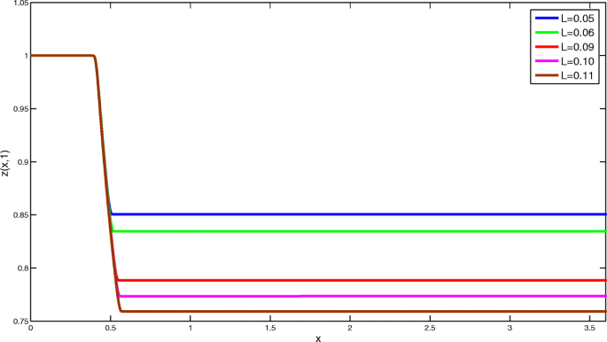

  

  Total fraction of unburnt gas inside the duct, varying the precatalyzer’s length, with r₂=0.04 m fixed

  Fig. 21

  

  Gas temperature inside the duct, varying the precatalyzer’s length, with r₂=0.04 m fixed

  Table 2 Total fraction of unburnt gas, maximum temperature, and volume, obtained varying the precatalyzer’s length, for a fixed radius r₁=0.04 m

  Note that, as one could expect, the longer the device, the longer the exposition time of the gas to the catalyzing substances, the smaller the total fraction of the unburnt gas. The temperature however increases, due to the honeycomb structure and to the chemical reactions occurring inside the precatalyzer. The same observations hold for the catalyzer, fixing its radius at the value r₂=0.06 m, and varying its length. The results are shown in Table 3.

  Table 3 Total fraction of unburnt gas, temperature, and volume, obtained varying the length for a fixed radius r₂=0.06 m

• Varying the radius. Let keep now fixed, instead, the precatalyzer’s length, L=0.09 m, and vary its radius. The results are qualitatively similar to those in Figs. 20, 21, and are summarized in Table 4. Note that (as is well known) increasing radius by a unity of a cylinder, its volume increases more significantly than increasing its length by the same amount.

  Table 4 Total fraction of unburnt gas, maximum temperature, and volume, obtained varying radius, for a fixed length L=0.09m

  As for the catalyzer, we fix its length L=0.07 m and vary its radius as was done for the precatalyzer. The most significant results are shown in the Table 5.

  Table 5 Total fraction of unburnt gas, maximum temperature, and volume, obtained varying catalyzer’s radius, for a fixed length L=0.07 m

Conclusions

Comparing the previous Tables, 2 and 4, one can observe that bigger volumes do not lead necessarily to better results. In fact, we found, e.g., that for r₁=0.04 m, L=0.05 m, and volume (of the whole catalyzer) V=0.00043 m³, the total fraction of unburnt gas is about equal to the third result in the third Table case above, Table 4, which corresponds to the values r₁=0.06 m, L=0.09 m, and V=0.00135 m³.

From Bernoulli equation,

$$ \frac{v^{2}}{2} + \frac{\gamma}{\gamma - 1} \, \frac{p}{\rho} = \text{const.}, $$

(18)

follows that a different pressure and thus a different temperature will affect the two catalyzers. In a catalyzer with a larger radius, the gas will exert a lower pressure with respect to another with smaller radius. Consequently, being the two physical quantities linked by the relation p=Rρθ, the temperature inside the first one will be lower than in the second one. (The temperature does not remain constant, but grows as pressure grows.)

The chemical reaction inside the catalyzer is governed by Arrhenius’ law, K(θ)=K₀ exp(−E⁺/θ), hence, when the temperature is very low, the reaction becomes negligible, and the source term in the fourth equation of the system of balance laws (8) essentially vanishes.

When two catalyzers have different volumes but yield similar results, it happens precisely this: the catalyzer with a larger radius, in order to provide the same result as the other (with a smaller radius), requires a higher exposition of the gas to the reacting substances, hence to be longer.

Therefore, one should choose a catalyzer with small radius, but sufficient length as to completely damp down the concentration of the noxious gas. However, such devices would be characterized by high temperatures. For instance, the first catalyzer in Table 4, has r₁=0.021 m (that is the radius of the pipe connecting the various parts). This was the best result we obtained, but the average and maximum temperatures are higher in such case.

Magneti Marelli provided temperature measurements at some points of the duct: for a motor’s temperature equal to 800 ^oC, these were never higher than about 1000 ^oC, while the maximum temperature attained by the device in question is about 1023 ^oC. All other catalyzers we considered attain lower temperatures. We conclude that the device set up by Magneti Marelli is indeed about the best. (Recall that for it, r₁=0.04 m and L=0.09 m.)

Similar considerations can be made for the catalyzer. The best result we obtained was that with L=0.07 m and r₂=0.04 m (see Table 5). Using these two devices together, a fraction of unburnt gas at the duct’s end about equal to 0.6859 was obtained, while for the Magneti Marelli device we have 0.7075. In Fig. 22, these two cases are compared, and on Fig. 23, the temperatures are compared.

Fig. 22

Comparing plots of the total fraction of unburnt gas inside the two ducts

Fig. 23

Comparing plots of the temperatures in the two ducts

References

Aregba-Driollet D, Natalini R (2000) Discrete Kinetic schemes for multidimensional conservation laws, SIAM. J Numer Anal 37:1973–2004.
Aregba-Driollet D, Briani M, Natalini R (2008) Asymptotic High-Order schemes for 2×2 dissipative hyperbolic systems, SIAM. J Numer Anal 46(2):869–894.
Briani M, Natalini R (2000) Asymptotic High-Order schemes for integro-differential problems arising in markets with jump, SIAM. J Numer 37(6):1973–2004.
Budzianowski WM, Miller R (2008) Auto-thermal combustion of lean gaseous fuels utilizing a recuperative annular double-layer catalytic converter. Can J Chem Eng 86:778–790.
Budzianowski WM, Miller R (2009) Superadiabatic lean catalytic combustion in a high-pressure reactor. Int J Chem React Eng 7:A20.
Budzianowski WM (2010) An oxy-fuel mass-recirculating process for H 2 production with C O 2capture by autothermal catalytic oxyforming of methane. Int J Hydrog Energy 35:7454–7469.
Chalapathi SK, Bhavanarayana Murthy Ch, Kumar BSP (2014) Development of automobile catalytic converter during last four decades. Int J Res Appl Sci Eng Techn 2:321–333.
Chen G-Q, Wagner DH (2003) Global entropy solutions to exothermically reacting, compressible Euler equations. J Diff Equat 191:277–322.
Dafermos CM, Hsiao L (1982) Hyperbolic systems of balance laws with inhomogeneity and dissipation, Indiana Univ. Math J 31:471–491.
Helzel C, Leveque RJ, Warnecke G (2000) A modified fractional step method for the accurate approximation of detonation waves, SIAM. J Sci Comput 22:1489–1510.
Kašpar J, Fornasiero P, Hickey N (2003) Automotive catalytic converters: current status and some perspectives. Catal Today 77:419–449.
Kurganov VA, Ibragimov MH. https://doi.org/10.1615/AtoZ.h.hydraulic_resistance. Accessed 16 Mar 2011.
Lacoste LMathematical modeling of chemical processes in exhaust pipe, Master Thesis, IAC - CNR, Rome, Years 2004-2005. [supervisor: R. Natalini].
Laidler KJ (1987) Chemical Kinetics, Harper and Row. 3rd Ed. Harper & Row, New York.
Sharma SK, Goyal P, Maheshwari S, Chandra AA technical review of automobile catalytic converter: current status and perspectives, Strategic Technologies of Complex Environmental Issues – A Sustainable Approac. ISBN: 978-93-83083-85-5. http://www.krishisanskriti.org/vol_image/10Sep201512090928.pdf.
Sweby PK (1984) High resolution schemes using flux limiters for hyperbolic conservation laws, SIAM. J Numer Anal 21(5):995–1011.
Acknowledgments
RS thanks his former student Roberta Petrucci, who carried out preliminary calculations concerning some duct’s profiles, and Roberto Natalini for very useful conversations. This work was partially (though not financially) supported by the GNFM of the Italian INdAM.
Availability of data and materials
Data sharing not applicable to this article as no datasets were generated or analyzed during the current study”.
Author information
Authors and Affiliations
Contributions
RS conceived the basic ideas of the paper and helped setting up the model. ML wrote the codes and ran them. ML and RS discussed together all results. Both authors read and approved the final manuscript.
Corresponding author
Ethics declarations
Ethics approval and consent to participate
Not applicable.
Consent for publication
Competing interests
The authors declare that they have no competing interests.
Publisher’s Note
Springer Nature remains neutral with regard to jurisdictional claims in published maps and institutional affiliations.
Rights and permissions
Open Access This article is distributed under the terms of the Creative Commons Attribution 4.0 International License (http://creativecommons.org/licenses/by/4.0/), which permits unrestricted use, distribution, and reproduction in any medium, provided you give appropriate credit to the original author(s) and the source, provide a link to the Creative Commons license, and indicate if changes were made.
About this article
Cite this article
Laurenzi, M., Spigler, R. Geometric effects in the design of catalytic converters in car exhaust pipes. Mathematics-in-Industry Case Studies 9, 1 (2018). https://doi.org/10.1186/s40929-018-0018-2
Received:
Accepted:
Published:
DOI: https://doi.org/10.1186/s40929-018-0018-2